Optimizing Average Precision Loss on Imbalanced CIFAR10 Dataset (SOAP)
Introduction
In this tutorial, you will learn how to quickly train a Resnet18
model by optimizing AUPRC with our novel APLoss and SOAP optimizer
[ref] on a binary image
classification task with CIFAR-10 dataset. After completion of this
tutorial, you should be able to use LibAUC to train your own models
on your own datasets.
Reference:
If you find this tutorial helpful in your work, please cite our library paper and the following papers:
@article{qi2021stochastic,
         title={Stochastic Optimization of Areas Under Precision-Recall Curves with Provable Convergence},
         author={Qi, Qi and Luo, Youzhi and Xu, Zhao and Ji, Shuiwang and Yang, Tianbao},
         journal={Advances in Neural Information Processing Systems},
         volume={34},
         year={2021}}
Install LibAUC
Let’s start with installing our library here. In this tutorial, we will use the lastest version for LibAUC by using pip install -U.
!pip install -U libauc
Importing LibAUC
Import required packages to use
from libauc.losses import APLoss
from libauc.optimizers import SOAP
from libauc.models import resnet18 as ResNet18
from libauc.datasets import CIFAR10
from libauc.utils import ImbalancedDataGenerator
from libauc.sampler import DualSampler
from libauc.metrics import auc_prc_score

import torchvision.transforms as transforms
from torch.utils.data import Dataset
import numpy as np
import torch
from PIL import Image
Reproducibility
The following function set_all_seeds limits the number of sources
of randomness behaviors, such as model intialization, data shuffling,
etcs. However, completely reproducible results are not guaranteed
across PyTorch releases
[Ref].
def set_all_seeds(SEED):
   # REPRODUCIBILITY
   np.random.seed(SEED)
   torch.manual_seed(SEED)
   torch.cuda.manual_seed(SEED)
   torch.backends.cudnn.deterministic = True
   torch.backends.cudnn.benchmark = False
set_all_seeds(2023)
Loading datasets
In this step, we will use the
CIFAR10 as
benchmark dataset. Before importing data to dataloader, we
construct imbalanced version for CIFAR10 by
ImbalanceDataGenerator. Specifically, it first randomly splits
the training data by class ID (e.g., 10 classes) into two even
portions as the positive and negative classes, and then it randomly
removes some samples from the positive class to make it imbalanced.
We keep the testing set untouched. We refer imratio to the ratio
of number of positive examples to number of all examples.
train_data, train_targets = CIFAR10(root='./data', train=True).as_array()
test_data, test_targets  = CIFAR10(root='./data', train=False).as_array()

imratio = 0.02  ## we set the imratio as 0.02 here since AP metric is usually used to evaluate highly imbalanced data.
generator = ImbalancedDataGenerator(verbose=True, random_seed=2023)
(train_images, train_labels) = generator.transform(train_data, train_targets, imratio=imratio)
(test_images, test_labels) = generator.transform(test_data, test_targets, imratio=0.5)
We define the data input pipeline such as data
augmentations. In this tutorial, we use RandomCrop,
RandomHorizontalFlip
class ImageDataset(Dataset):
   def __init__(self, images, targets, image_size=32, crop_size=30, mode='train'):
      self.images = images.astype(np.uint8)
      self.targets = targets
      self.mode = mode
      self.transform_train = transforms.Compose([
                              transforms.ToTensor(),
                              transforms.RandomCrop((crop_size, crop_size), padding=None),
                              transforms.RandomHorizontalFlip(),
                              transforms.Resize((image_size, image_size), antialias=True),
                              ])
      self.transform_test = transforms.Compose([
                           transforms.ToTensor(),
                           transforms.Resize((image_size, image_size), antialias=True),
                              ])
   def __len__(self):
      return len(self.images)

   def __getitem__(self, idx):
      image = self.images[idx]
      target = self.targets[idx]
      image = Image.fromarray(image.astype('uint8'))
      if self.mode == 'train':
            image = self.transform_train(image)
      else:
            image = self.transform_test(image)
      return image, target, idx
Configuration
Hyper-Parameters
# Hyper-Parameters
lr = 1e-3
margin = 0.6
gamma = 0.1
weight_decay = 2e-4
total_epoch = 60
decay_epoch = [30, 45]
load_pretrain = False
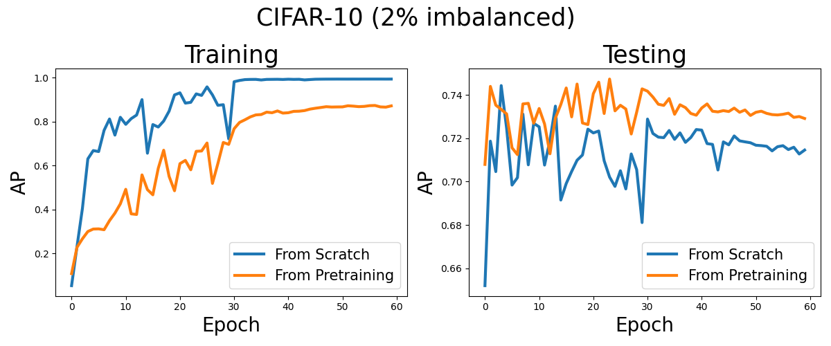
Pretraining (Recommended)
Following the original paper, it’s recommended to start from a pretrained checkpoint with cross-entropy loss to significantly boost models’ performance. It includes a pre-training step with standard cross-entropy loss, and an AUPRC maximization step that maximizes an AUPRC surrogate loss of the pre-trained model.
from torch.optim import Adam
import warnings
warnings.filterwarnings('ignore')

load_pretrain = True
model = ResNet18(pretrained=False, last_activation=None, num_classes=1)
model = model.cuda()

loss_fn = torch.nn.BCELoss()
optimizer =Adam(model.parameters(), lr=lr, weight_decay=weight_decay)

trainloader = torch.utils.data.DataLoader(trainSet, batch_size=batch_size, shuffle=True, num_workers=2)
testloader = torch.utils.data.DataLoader(testSet, batch_size=batch_size, shuffle=False, num_workers=2)


best_test = 0
for epoch in range(total_epoch):
   if epoch in decay_epoch:
      for param_group in optimizer.param_groups:
            param_group['lr'] = 0.1 * param_group['lr']

   model.train()
   for idx, (data, targets, index) in enumerate(trainloader):
      data, targets, index  = data.cuda(), targets.cuda(), index.cuda()
      y_pred = model(data)
      y_prob = torch.sigmoid(y_pred)
      loss = loss_fn(y_prob, targets)
      optimizer.zero_grad()
      loss.backward()
      optimizer.step()

   ######***evaluation***####
   # evaluation on test sets
   model.eval()
   test_pred_list, test_true_list = [], []
   with torch.no_grad():
      for j, data in enumerate(testloader):
         test_data, test_targets, _ = data
         test_data = test_data.cuda()
         y_pred = model(test_data)
         y_prob = torch.sigmoid(y_pred)
         test_pred_list.append(y_prob.cpu().detach().numpy())
         test_true_list.append(test_targets.numpy())
   test_true = np.concatenate(test_true_list)
   test_pred = np.concatenate(test_pred_list)

   test_ap = auc_prc_score(test_true, test_pred)
   if best_test < test_ap:
      best_test = test_ap
      torch.save(model.state_dict(), 'ce_pretrained_model_soap.pth')

   model.train()
   print("epoch: %s, test_ap: %.4f, best_test_ap: %.4f, lr: %.4f"%(epoch, test_ap, best_test, optimizer.param_groups[0]['lr'] ))
epoch: 0, test_ap: 0.5846, best_test_ap: 0.5846, lr: 0.0010
epoch: 1, test_ap: 0.5718, best_test_ap: 0.5846, lr: 0.0010
epoch: 2, test_ap: 0.5325, best_test_ap: 0.5846, lr: 0.0010
epoch: 3, test_ap: 0.5308, best_test_ap: 0.5846, lr: 0.0010
epoch: 4, test_ap: 0.5789, best_test_ap: 0.5846, lr: 0.0010
epoch: 5, test_ap: 0.5702, best_test_ap: 0.5846, lr: 0.0010
epoch: 6, test_ap: 0.5875, best_test_ap: 0.5875, lr: 0.0010
epoch: 7, test_ap: 0.5230, best_test_ap: 0.5875, lr: 0.0010
epoch: 8, test_ap: 0.5039, best_test_ap: 0.5875, lr: 0.0010
epoch: 9, test_ap: 0.5245, best_test_ap: 0.5875, lr: 0.0010
epoch: 10, test_ap: 0.5678, best_test_ap: 0.5875, lr: 0.0010
epoch: 11, test_ap: 0.5451, best_test_ap: 0.5875, lr: 0.0010
epoch: 12, test_ap: 0.5458, best_test_ap: 0.5875, lr: 0.0010
epoch: 13, test_ap: 0.5509, best_test_ap: 0.5875, lr: 0.0010
epoch: 14, test_ap: 0.5686, best_test_ap: 0.5875, lr: 0.0010
epoch: 15, test_ap: 0.5714, best_test_ap: 0.5875, lr: 0.0010
epoch: 16, test_ap: 0.6056, best_test_ap: 0.6056, lr: 0.0010
epoch: 17, test_ap: 0.6154, best_test_ap: 0.6154, lr: 0.0010
epoch: 18, test_ap: 0.6038, best_test_ap: 0.6154, lr: 0.0010
epoch: 19, test_ap: 0.6239, best_test_ap: 0.6239, lr: 0.0010
epoch: 20, test_ap: 0.6115, best_test_ap: 0.6239, lr: 0.0010
epoch: 21, test_ap: 0.6245, best_test_ap: 0.6245, lr: 0.0010
epoch: 22, test_ap: 0.6366, best_test_ap: 0.6366, lr: 0.0010
epoch: 23, test_ap: 0.6179, best_test_ap: 0.6366, lr: 0.0010
epoch: 24, test_ap: 0.6395, best_test_ap: 0.6395, lr: 0.0010
epoch: 25, test_ap: 0.6070, best_test_ap: 0.6395, lr: 0.0010
epoch: 26, test_ap: 0.6396, best_test_ap: 0.6396, lr: 0.0010
epoch: 27, test_ap: 0.6377, best_test_ap: 0.6396, lr: 0.0010
epoch: 28, test_ap: 0.6509, best_test_ap: 0.6509, lr: 0.0010
epoch: 29, test_ap: 0.6425, best_test_ap: 0.6509, lr: 0.0010
epoch: 30, test_ap: 0.6614, best_test_ap: 0.6614, lr: 0.0001
epoch: 31, test_ap: 0.6650, best_test_ap: 0.6650, lr: 0.0001
epoch: 32, test_ap: 0.6735, best_test_ap: 0.6735, lr: 0.0001
epoch: 33, test_ap: 0.6772, best_test_ap: 0.6772, lr: 0.0001
epoch: 34, test_ap: 0.6775, best_test_ap: 0.6775, lr: 0.0001
epoch: 35, test_ap: 0.6847, best_test_ap: 0.6847, lr: 0.0001
epoch: 36, test_ap: 0.6877, best_test_ap: 0.6877, lr: 0.0001
epoch: 37, test_ap: 0.6868, best_test_ap: 0.6877, lr: 0.0001
epoch: 38, test_ap: 0.6902, best_test_ap: 0.6902, lr: 0.0001
epoch: 39, test_ap: 0.6894, best_test_ap: 0.6902, lr: 0.0001
epoch: 40, test_ap: 0.6998, best_test_ap: 0.6998, lr: 0.0001
epoch: 41, test_ap: 0.6913, best_test_ap: 0.6998, lr: 0.0001
epoch: 42, test_ap: 0.6868, best_test_ap: 0.6998, lr: 0.0001
epoch: 43, test_ap: 0.7004, best_test_ap: 0.7004, lr: 0.0001
epoch: 44, test_ap: 0.7087, best_test_ap: 0.7087, lr: 0.0001
epoch: 45, test_ap: 0.7070, best_test_ap: 0.7087, lr: 0.0000
epoch: 46, test_ap: 0.7080, best_test_ap: 0.7087, lr: 0.0000
epoch: 47, test_ap: 0.7083, best_test_ap: 0.7087, lr: 0.0000
epoch: 48, test_ap: 0.7092, best_test_ap: 0.7092, lr: 0.0000
epoch: 49, test_ap: 0.7086, best_test_ap: 0.7092, lr: 0.0000
epoch: 50, test_ap: 0.7092, best_test_ap: 0.7092, lr: 0.0000
epoch: 51, test_ap: 0.7100, best_test_ap: 0.7100, lr: 0.0000
epoch: 52, test_ap: 0.7090, best_test_ap: 0.7100, lr: 0.0000
epoch: 53, test_ap: 0.7099, best_test_ap: 0.7100, lr: 0.0000
epoch: 54, test_ap: 0.7093, best_test_ap: 0.7100, lr: 0.0000
epoch: 55, test_ap: 0.7104, best_test_ap: 0.7104, lr: 0.0000
epoch: 56, test_ap: 0.7109, best_test_ap: 0.7109, lr: 0.0000
epoch: 57, test_ap: 0.7115, best_test_ap: 0.7115, lr: 0.0000
epoch: 58, test_ap: 0.7124, best_test_ap: 0.7124, lr: 0.0000
epoch: 59, test_ap: 0.7128, best_test_ap: 0.7128, lr: 0.0000
Optimizing AUPRC Loss
We define dataset, DualSampler and dataloader here. By
default, we use batch_size 64 and we oversample the minority
class with pos:neg=1:1 by setting sampling_rate=0.5.
sampling_rate = 0.5

sampler = DualSampler(trainSet, batch_size, sampling_rate=sampling_rate)
trainloader = torch.utils.data.DataLoader(trainSet, batch_size=batch_size, sampler=sampler, num_workers=2)
trainloader_eval = torch.utils.data.DataLoader(trainSet_eval, batch_size=batch_size, shuffle=False, num_workers=2)
testloader = torch.utils.data.DataLoader(testSet, batch_size=batch_size, shuffle=False, num_workers=2)
Model, Loss and Optimizer
model = ResNet18(pretrained=False, last_activation=None, num_classes=1)
model = model.cuda()
# load pretrained model
if load_pretrain:
   PATH = 'ce_pretrained_model_soap.pth'
   state_dict = torch.load(PATH)
   filtered = {k:v for k,v in state_dict.items() if 'fc' not in k}
   msg = model.load_state_dict(filtered, False)
   print(msg)
   model.fc.reset_parameters()

loss_fn = APLoss(data_len=len(trainSet), margin=margin, gamma=gamma)
optimizer = SOAP(model.parameters(), lr=lr, mode='adam', weight_decay=weight_decay)
Training
Now it’s time for training. And we evaluate Average Precision performance after every epoch.
print ('Start Training')
print ('-'*30)

train_log, test_log = [], []
best_test = 0
for epoch in range(total_epoch):
   if epoch in decay_epoch:
      optimizer.update_lr(decay_factor=10)

   model.train()
   for idx, (data, targets, index) in enumerate(trainloader):
      data, targets, index  = data.cuda(), targets.cuda(), index.cuda()
      y_pred = model(data)
      y_prob = torch.sigmoid(y_pred)
      loss = loss_fn(y_prob, targets, index)
      optimizer.zero_grad()
      loss.backward()
      optimizer.step()

   ######***evaluation***####
   # evaluation on training sets
   model.eval()
   train_pred_list, train_true_list = [], []
   with torch.no_grad():
      for i, data in enumerate(trainloader_eval):
            train_data, train_targets, _ = data
            train_data = train_data.cuda()
            y_pred = model(train_data)
            y_prob = torch.sigmoid(y_pred)
            train_pred_list.append(y_prob.cpu().detach().numpy())
            train_true_list.append(train_targets.cpu().detach().numpy())
   train_true = np.concatenate(train_true_list)
   train_pred = np.concatenate(train_pred_list)

   train_ap = auc_prc_score(train_true, train_pred)
   train_log.append(train_ap)

   # evaluation on test sets
   model.eval()
   test_pred_list, test_true_list = [], []
   with torch.no_grad():
      for j, data in enumerate(testloader):
            test_data, test_targets, _ = data
            test_data = test_data.cuda()
            y_pred = model(test_data)
            y_prob = torch.sigmoid(y_pred)
            test_pred_list.append(y_prob.cpu().detach().numpy())
            test_true_list.append(test_targets.numpy())
   test_true = np.concatenate(test_true_list)
   test_pred = np.concatenate(test_pred_list)

   test_ap = auc_prc_score(test_true, test_pred)
   test_log.append(test_ap)
   if best_test < test_ap:
      best_test = test_ap

   model.train()
   print("epoch: %s, train_ap: %.4f, test_ap: %.4f, best_test_ap: %.4f, lr: %.4f"%(epoch, train_ap, test_ap, best_test, optimizer.lr ))
Start Training
------------------------------
epoch: 0, train_ap: 0.1086, test_ap: 0.7079, best_test_ap: 0.7079, lr: 0.0010
epoch: 1, train_ap: 0.2284, test_ap: 0.7439, best_test_ap: 0.7439, lr: 0.0010
epoch: 2, train_ap: 0.2671, test_ap: 0.7353, best_test_ap: 0.7439, lr: 0.0010
epoch: 3, train_ap: 0.3002, test_ap: 0.7333, best_test_ap: 0.7439, lr: 0.0010
epoch: 4, train_ap: 0.3115, test_ap: 0.7312, best_test_ap: 0.7439, lr: 0.0010
epoch: 5, train_ap: 0.3123, test_ap: 0.7156, best_test_ap: 0.7439, lr: 0.0010
epoch: 6, train_ap: 0.3084, test_ap: 0.7125, best_test_ap: 0.7439, lr: 0.0010
epoch: 7, train_ap: 0.3497, test_ap: 0.7358, best_test_ap: 0.7439, lr: 0.0010
epoch: 8, train_ap: 0.3840, test_ap: 0.7361, best_test_ap: 0.7439, lr: 0.0010
epoch: 9, train_ap: 0.4262, test_ap: 0.7269, best_test_ap: 0.7439, lr: 0.0010
epoch: 10, train_ap: 0.4925, test_ap: 0.7337, best_test_ap: 0.7439, lr: 0.0010
epoch: 11, train_ap: 0.3807, test_ap: 0.7266, best_test_ap: 0.7439, lr: 0.0010
epoch: 12, train_ap: 0.3779, test_ap: 0.7128, best_test_ap: 0.7439, lr: 0.0010
epoch: 13, train_ap: 0.5582, test_ap: 0.7293, best_test_ap: 0.7439, lr: 0.0010
epoch: 14, train_ap: 0.4909, test_ap: 0.7356, best_test_ap: 0.7439, lr: 0.0010
epoch: 15, train_ap: 0.4674, test_ap: 0.7432, best_test_ap: 0.7439, lr: 0.0010
epoch: 16, train_ap: 0.5882, test_ap: 0.7299, best_test_ap: 0.7439, lr: 0.0010
epoch: 17, train_ap: 0.6705, test_ap: 0.7450, best_test_ap: 0.7450, lr: 0.0010
epoch: 18, train_ap: 0.5512, test_ap: 0.7270, best_test_ap: 0.7450, lr: 0.0010
epoch: 19, train_ap: 0.4859, test_ap: 0.7263, best_test_ap: 0.7450, lr: 0.0010
epoch: 20, train_ap: 0.6092, test_ap: 0.7405, best_test_ap: 0.7450, lr: 0.0010
epoch: 21, train_ap: 0.6242, test_ap: 0.7459, best_test_ap: 0.7459, lr: 0.0010
epoch: 22, train_ap: 0.5813, test_ap: 0.7314, best_test_ap: 0.7459, lr: 0.0010
epoch: 23, train_ap: 0.6655, test_ap: 0.7473, best_test_ap: 0.7473, lr: 0.0010
epoch: 24, train_ap: 0.6669, test_ap: 0.7326, best_test_ap: 0.7473, lr: 0.0010
epoch: 25, train_ap: 0.7032, test_ap: 0.7352, best_test_ap: 0.7473, lr: 0.0010
epoch: 26, train_ap: 0.5194, test_ap: 0.7335, best_test_ap: 0.7473, lr: 0.0010
epoch: 27, train_ap: 0.6097, test_ap: 0.7220, best_test_ap: 0.7473, lr: 0.0010
epoch: 28, train_ap: 0.7058, test_ap: 0.7320, best_test_ap: 0.7473, lr: 0.0010
epoch: 29, train_ap: 0.6970, test_ap: 0.7428, best_test_ap: 0.7473, lr: 0.0010
Reducing learning rate to 0.00010 @ T=23430!
epoch: 30, train_ap: 0.7684, test_ap: 0.7417, best_test_ap: 0.7473, lr: 0.0001
epoch: 31, train_ap: 0.7969, test_ap: 0.7390, best_test_ap: 0.7473, lr: 0.0001
epoch: 32, train_ap: 0.8090, test_ap: 0.7357, best_test_ap: 0.7473, lr: 0.0001
epoch: 33, train_ap: 0.8223, test_ap: 0.7352, best_test_ap: 0.7473, lr: 0.0001
epoch: 34, train_ap: 0.8312, test_ap: 0.7383, best_test_ap: 0.7473, lr: 0.0001
epoch: 35, train_ap: 0.8329, test_ap: 0.7311, best_test_ap: 0.7473, lr: 0.0001
epoch: 36, train_ap: 0.8438, test_ap: 0.7354, best_test_ap: 0.7473, lr: 0.0001
epoch: 37, train_ap: 0.8411, test_ap: 0.7341, best_test_ap: 0.7473, lr: 0.0001
epoch: 38, train_ap: 0.8493, test_ap: 0.7314, best_test_ap: 0.7473, lr: 0.0001
epoch: 39, train_ap: 0.8395, test_ap: 0.7306, best_test_ap: 0.7473, lr: 0.0001
epoch: 40, train_ap: 0.8411, test_ap: 0.7339, best_test_ap: 0.7473, lr: 0.0001
epoch: 41, train_ap: 0.8473, test_ap: 0.7358, best_test_ap: 0.7473, lr: 0.0001
epoch: 42, train_ap: 0.8480, test_ap: 0.7325, best_test_ap: 0.7473, lr: 0.0001
epoch: 43, train_ap: 0.8510, test_ap: 0.7322, best_test_ap: 0.7473, lr: 0.0001
epoch: 44, train_ap: 0.8575, test_ap: 0.7327, best_test_ap: 0.7473, lr: 0.0001
Reducing learning rate to 0.00001 @ T=35145!
epoch: 45, train_ap: 0.8616, test_ap: 0.7323, best_test_ap: 0.7473, lr: 0.0000
epoch: 46, train_ap: 0.8650, test_ap: 0.7339, best_test_ap: 0.7473, lr: 0.0000
epoch: 47, train_ap: 0.8686, test_ap: 0.7320, best_test_ap: 0.7473, lr: 0.0000
epoch: 48, train_ap: 0.8670, test_ap: 0.7331, best_test_ap: 0.7473, lr: 0.0000
epoch: 49, train_ap: 0.8675, test_ap: 0.7305, best_test_ap: 0.7473, lr: 0.0000
epoch: 50, train_ap: 0.8677, test_ap: 0.7320, best_test_ap: 0.7473, lr: 0.0000
epoch: 51, train_ap: 0.8728, test_ap: 0.7325, best_test_ap: 0.7473, lr: 0.0000
epoch: 52, train_ap: 0.8712, test_ap: 0.7315, best_test_ap: 0.7473, lr: 0.0000
epoch: 53, train_ap: 0.8688, test_ap: 0.7309, best_test_ap: 0.7473, lr: 0.0000
epoch: 54, train_ap: 0.8700, test_ap: 0.7308, best_test_ap: 0.7473, lr: 0.0000
epoch: 55, train_ap: 0.8733, test_ap: 0.7310, best_test_ap: 0.7473, lr: 0.0000
epoch: 56, train_ap: 0.8742, test_ap: 0.7316, best_test_ap: 0.7473, lr: 0.0000
epoch: 57, train_ap: 0.8677, test_ap: 0.7296, best_test_ap: 0.7473, lr: 0.0000
epoch: 58, train_ap: 0.8666, test_ap: 0.7300, best_test_ap: 0.7473, lr: 0.0000
epoch: 59, train_ap: 0.8723, test_ap: 0.7291, best_test_ap: 0.7473, lr: 0.0000
Visualization
Now, let’s see the learning curves for optimizing AUPRC on train and test sets.
import matplotlib.pyplot as plt

train_log_scratch = [0.053795023112763615, 0.23188408521453444, 0.40498580476379314, 0.6309250870453721, 0.6688097705145062, 0.6643704133362177, 0.7609703897219161, 0.8126110098607636, 0.7391549531236978, 0.8203093897564716, 0.7882754483018704, 0.8141741351522646, 0.8305163466394554, 0.9009450492503674, 0.656848716147405, 0.7873017198831529, 0.7759555212411272, 0.8034168454598932, 0.8483244157244562, 0.9222037489554733, 0.9317955898559406, 0.8847965985232369, 0.8884650540237902, 0.926951756700307, 0.919984223429547, 0.958945851785437, 0.9224273413498014, 0.874809468705223, 0.8776531193301593, 0.7221880777702656, 0.9823628544780301, 0.988045111478341, 0.9919440943863796, 0.9927644846117613, 0.9929448560903278, 0.9902814488208145, 0.992806164193639, 0.9930282561755731, 0.9933296962549633, 0.9925766632457378, 0.9936864759528751, 0.9929546646584996, 0.9933665270309218, 0.9906275286274027, 0.9921974812223809, 0.9936407755498231, 0.9939732471875866, 0.994189589656222, 0.9942241268264275, 0.9943356450235398, 0.9942766903363517, 0.9942551172502118, 0.9943444210686041, 0.9943006306769221, 0.9943708434068441, 0.9943799172038008, 0.9943891711503321, 0.994388939404161, 0.9942857595863284, 0.9943904925225493]
test_log_scratch = [0.6520089832395508, 0.7186568242083518, 0.7046210471940082, 0.7442952936880263, 0.7245767873876033, 0.6984044779997952, 0.7018429018958507, 0.7311436349021154, 0.7077461028919111, 0.7268788584445507, 0.7252711333916387, 0.7076312487047431, 0.7190415396093803, 0.7348218283409199, 0.6914963088184523, 0.6991144030721776, 0.7046812298764077, 0.709850114220171, 0.7122859049382089, 0.7241964658929886, 0.7224599388035504, 0.723338839441545, 0.7096185435770437, 0.7021200123558938, 0.6977969912638463, 0.7050140616518277, 0.6966216205469574, 0.7127619213599601, 0.705529722176301, 0.6811019253316897, 0.7288481832683131, 0.7221896161787591, 0.7205241991504794, 0.7202767183319769, 0.7235876734810258, 0.7194841647258248, 0.7224814210889982, 0.7181062100088227, 0.7203680443941286, 0.7240232613107201, 0.7237644398520424, 0.7175346947972038, 0.7171679960385751, 0.7053624508699083, 0.7183287385368646, 0.7169735008795999, 0.7210729985374514, 0.7187984764180114, 0.7183434767791061, 0.717924818866893, 0.7167852808359665, 0.7165983652485299, 0.716295569959561, 0.7141804015908193, 0.7161031523724993, 0.7165712767282505, 0.7147814607909024, 0.7158626888548612, 0.7127440037152936, 0.7145540619518064]

# plt.rcParams["figure.figsize"] = (9,5)
fig, (ax0, ax1) = plt.subplots(1, 2, figsize=(12,5))
plt.suptitle('CIFAR-10 (2% imbalanced)',fontsize=25)

x=np.arange(len(train_log))
ax0.plot(x, train_log_scratch,  label='From Scratch', linewidth=3)
ax0.plot(x, train_log,  label='From Pretraining', linewidth=3)
ax0.set_title('Training',fontsize=25)
ax1.plot(x, test_log_scratch, label='From Scratch', linewidth=3)
ax1.plot(x, test_log, label='From Pretraining', linewidth=3)
ax1.set_title('Testing',fontsize=25)

ax0.legend(fontsize=15)
ax1.legend(fontsize=15)
ax0.set_ylabel('AP', fontsize=20)
ax0.set_xlabel('Epoch', fontsize=20)
ax1.set_ylabel('AP', fontsize=20)
ax1.set_xlabel('Epoch', fontsize=20)

plt.tight_layout()
plt.show()
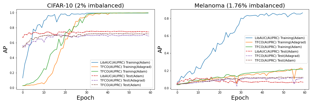
Comparison
Furthermore, we compare our library with TensorFlow Constrained Optimization (TFCO) library which can also be used to maximize AUPRC. For more information about TensorFlow Constrained Optimization (TFCO), please refer to this link [Ref]. In the comparative experiment, we all train from scratch with same dataset, network and data augmentation. Although TFCO tutorial adopts Adagrad as the default optimizer, we also conduct experiment with Adam optimizer for fair comparison.