Optimizing Two-Way partial AUC on Imbalanced CIFAR10 Dataset (SOTAs)
Introduction
In this tutorial, we will learn how to quickly train a ResNet18 model by optimizing two way partial AUC (TPAUC) score using our novel tpAUC_KL_Loss and SOTAs optimizer [Ref] method on a binary image classification task on Cifar10. After completion of this tutorial, you should be able to use LibAUC to train your own models on your own datasets.
Reference:
If you find this tutorial helpful in your work, please cite our [library paper] and the following papers:
@inproceedings{zhu2022auc,
               title={When auc meets dro: Optimizing partial auc for deep learning with non-convex convergence guarantee},
               author={Zhu, Dixian and Li, Gang and Wang, Bokun and Wu, Xiaodong and Yang, Tianbao},
               booktitle={International Conference on Machine Learning},
               pages={27548--27573},
               year={2022},
               organization={PMLR}
             }
Install LibAUC
Let’s start with installing our library here. In this tutorial, we will use the lastest version for LibAUC by using pip install -U.
!pip install -U libauc
Importing LibAUC
Import required libraries to use
from libauc.models import resnet18
from libauc.datasets import CIFAR10
from libauc.losses import tpAUC_KL_Loss
from libauc.optimizers import SOTAs
from libauc.utils import ImbalancedDataGenerator
from libauc.sampler import DualSampler # data resampling (for binary class)
from libauc.metrics import pauc_roc_score

import torch
from PIL import Image
import numpy as np
import torchvision.transforms as transforms
from torch.utils.data import Dataset
Reproducibility
The following function set_all_seeds limits the number of sources
of randomness behaviors, such as model intialization, data shuffling,
etcs. However, completely reproducible results are not guaranteed
across PyTorch releases
[Ref].
def set_all_seeds(SEED):
   # REPRODUCIBILITY
   np.random.seed(SEED)
   torch.manual_seed(SEED)
   torch.cuda.manual_seed(SEED)
   torch.backends.cudnn.deterministic = True
   torch.backends.cudnn.benchmark = False
set_all_seeds(2023)
Image Dataset
Now we define the data input pipeline such as data augmentations. In this tutorials, we use RandomCrop, RandomHorizontalFlip. The pos_index_map helps map global index to local index for reducing memory cost in loss function since we only need to track the indices for positive samples.
class ImageDataset(Dataset):
  def __init__(self, images, targets, image_size=32, crop_size=30, mode='train'):
    self.images = images.astype(np.uint8)
    self.targets = targets
    self.mode = mode
    self.transform_train = transforms.Compose([
                            transforms.ToTensor(),
                            transforms.RandomCrop((crop_size, crop_size), padding=None),
                            transforms.RandomHorizontalFlip(),
                            transforms.Resize((image_size, image_size)),
                            ])
    self.transform_test = transforms.Compose([
                          transforms.ToTensor(),
                          transforms.Resize((image_size, image_size)),
                            ])

    # for loss function
    self.pos_indices = np.flatnonzero(targets==1)
    self.pos_index_map = {}
    for i, idx in enumerate(self.pos_indices):
        self.pos_index_map[idx] = i

  def __len__(self):
      return len(self.images)

  def __getitem__(self, idx):
      image = self.images[idx]
      target = self.targets[idx]
      image = Image.fromarray(image.astype('uint8'))
      if self.mode == 'train':
          idx = self.pos_index_map[idx] if idx in self.pos_indices else -1
          image = self.transform_train(image)
      else:
          image = self.transform_test(image)
      return image, target, idx
HyperParameters
# HyperParameters
SEED = 123
batch_size = 64
total_epochs = 60
weight_decay = 2e-4
lr = 1e-3
decay_epochs = [30, 45]
decay_factor = 10

gamma0 = 0.5 # learning rate for control negative samples weights
gamma1 = 0.5 # learning rate for control positive samples weights

tau = 1.0 # KL-DRO regularization for outer positive samples part  #
Lambda = 0.5 # KL-DRO regularization for inner negative samples part #
load_pretrain = False
Loading datasets
# load data as numpy arrays
train_data, train_targets = CIFAR10(root='./data', train=True).as_array()
test_data, test_targets  = CIFAR10(root='./data', train=False).as_array()

# generate imbalanced data
imratio = 0.2
generator = ImbalancedDataGenerator(shuffle=True, verbose=True, random_seed=2023)
(train_images, train_labels) = generator.transform(train_data, train_targets, imratio=imratio)
(test_images, test_labels) = generator.transform(test_data, test_targets, imratio=imratio)

# data augmentations
trainDataset = ImageDataset(train_images, train_labels)
testDataset = ImageDataset(test_images, test_labels, mode='test')
Downloading https://www.cs.toronto.edu/~kriz/cifar-10-python.tar.gz to ./data/cifar-10-python.tar.gz
  0%|          | 0/170498071 [00:00<?, ?it/s]
Extracting ./data/cifar-10-python.tar.gz to ./data
Files already downloaded and verified
#SAMPLES: 31250, CLASS 0.0 COUNT: 25000, CLASS RATIO: 0.8000
#SAMPLES: 31250, CLASS 1.0 COUNT: 6250, CLASS RATIO: 0.2000
#SAMPLES: 6250, CLASS 0.0 COUNT: 5000, CLASS RATIO: 0.8000
#SAMPLES: 6250, CLASS 1.0 COUNT: 1250, CLASS RATIO: 0.2000
Pretraining (Recommended)
Following the original paper, it’s recommended to start from a pretrained checkpoint with cross-entropy loss to significantly boost models’ performance. It includes a pre-training step with standard cross-entropy loss, and a Partial AUC maximization step that maximizes a Partial AUC surrogate loss of the pre-trained model.
from torch.optim import Adam
import warnings
warnings.filterwarnings('ignore')

load_pretrain = True
model = resnet18(pretrained=False, num_classes=1, last_activation=None)
model = model.cuda()

loss_fn = torch.nn.BCELoss()
optimizer =Adam(model.parameters(), lr=lr, weight_decay=weight_decay)

trainloader = torch.utils.data.DataLoader(trainDataset, batch_size=batch_size, shuffle=True, num_workers=2)
testloader = torch.utils.data.DataLoader(testDataset, batch_size=batch_size, shuffle=False, num_workers=2)


best_test = 0
for epoch in range(total_epochs):
    if epoch in decay_epochs:
        for param_group in optimizer.param_groups:
            param_group['lr'] = 0.1 * param_group['lr']

    model.train()
    for idx, (data, targets, index) in enumerate(trainloader):
        data, targets, index  = data.cuda(), targets.cuda(), index.cuda()
        y_pred = model(data)
        y_prob = torch.sigmoid(y_pred)
        loss = loss_fn(y_prob, targets)
        optimizer.zero_grad()
        loss.backward()
        optimizer.step()

    ######***evaluation***####
    # evaluation on test sets
    model.eval()
    test_pred_list, test_true_list = [], []
    with torch.no_grad():
        for j, data in enumerate(testloader):
            test_data, test_targets, _ = data
            test_data = test_data.cuda()
            y_pred = model(test_data)
            y_prob = torch.sigmoid(y_pred)
            test_pred_list.append(y_prob.cpu().detach().numpy())
            test_true_list.append(test_targets.numpy())
    test_true = np.concatenate(test_true_list)
    test_pred = np.concatenate(test_pred_list)

    test_pauc = pauc_roc_score(test_true, test_pred, max_fpr = 0.3, min_tpr=0.7)
    if best_test < test_pauc:
        best_test = test_pauc
        torch.save(model.state_dict(), 'ce_pretrained_model_sotas.pth')

    model.train()
    print("epoch: %s, test_pauc: %.4f, best_test_pauc: %.4f, lr: %.4f"%(epoch, test_pauc, best_test, optimizer.param_groups[0]['lr'] ))
epoch: 0, test_pauc: 0.0000, best_test_pauc: 0.0000, lr: 0.0010
epoch: 1, test_pauc: 0.0000, best_test_pauc: 0.0000, lr: 0.0010
epoch: 2, test_pauc: 0.0000, best_test_pauc: 0.0000, lr: 0.0010
epoch: 3, test_pauc: 0.0015, best_test_pauc: 0.0015, lr: 0.0010
epoch: 4, test_pauc: 0.0000, best_test_pauc: 0.0015, lr: 0.0010
epoch: 5, test_pauc: 0.0006, best_test_pauc: 0.0015, lr: 0.0010
epoch: 6, test_pauc: 0.0462, best_test_pauc: 0.0462, lr: 0.0010
epoch: 7, test_pauc: 0.0452, best_test_pauc: 0.0462, lr: 0.0010
epoch: 8, test_pauc: 0.0648, best_test_pauc: 0.0648, lr: 0.0010
epoch: 9, test_pauc: 0.0502, best_test_pauc: 0.0648, lr: 0.0010
epoch: 10, test_pauc: 0.0223, best_test_pauc: 0.0648, lr: 0.0010
epoch: 11, test_pauc: 0.1365, best_test_pauc: 0.1365, lr: 0.0010
epoch: 12, test_pauc: 0.1835, best_test_pauc: 0.1835, lr: 0.0010
epoch: 13, test_pauc: 0.1504, best_test_pauc: 0.1835, lr: 0.0010
epoch: 14, test_pauc: 0.1309, best_test_pauc: 0.1835, lr: 0.0010
epoch: 15, test_pauc: 0.1324, best_test_pauc: 0.1835, lr: 0.0010
epoch: 16, test_pauc: 0.0902, best_test_pauc: 0.1835, lr: 0.0010
epoch: 17, test_pauc: 0.2067, best_test_pauc: 0.2067, lr: 0.0010
epoch: 18, test_pauc: 0.1518, best_test_pauc: 0.2067, lr: 0.0010
epoch: 19, test_pauc: 0.2301, best_test_pauc: 0.2301, lr: 0.0010
epoch: 20, test_pauc: 0.2029, best_test_pauc: 0.2301, lr: 0.0010
epoch: 21, test_pauc: 0.2525, best_test_pauc: 0.2525, lr: 0.0010
epoch: 22, test_pauc: 0.2781, best_test_pauc: 0.2781, lr: 0.0010
epoch: 23, test_pauc: 0.1905, best_test_pauc: 0.2781, lr: 0.0010
epoch: 24, test_pauc: 0.2337, best_test_pauc: 0.2781, lr: 0.0010
epoch: 25, test_pauc: 0.2410, best_test_pauc: 0.2781, lr: 0.0010
epoch: 26, test_pauc: 0.2799, best_test_pauc: 0.2799, lr: 0.0010
epoch: 27, test_pauc: 0.1634, best_test_pauc: 0.2799, lr: 0.0010
epoch: 28, test_pauc: 0.2501, best_test_pauc: 0.2799, lr: 0.0010
epoch: 29, test_pauc: 0.2819, best_test_pauc: 0.2819, lr: 0.0010
epoch: 30, test_pauc: 0.3268, best_test_pauc: 0.3268, lr: 0.0001
epoch: 31, test_pauc: 0.3304, best_test_pauc: 0.3304, lr: 0.0001
epoch: 32, test_pauc: 0.3261, best_test_pauc: 0.3304, lr: 0.0001
epoch: 33, test_pauc: 0.3293, best_test_pauc: 0.3304, lr: 0.0001
epoch: 34, test_pauc: 0.3196, best_test_pauc: 0.3304, lr: 0.0001
epoch: 35, test_pauc: 0.3338, best_test_pauc: 0.3338, lr: 0.0001
epoch: 36, test_pauc: 0.3135, best_test_pauc: 0.3338, lr: 0.0001
epoch: 37, test_pauc: 0.3449, best_test_pauc: 0.3449, lr: 0.0001
epoch: 38, test_pauc: 0.3290, best_test_pauc: 0.3449, lr: 0.0001
epoch: 39, test_pauc: 0.3378, best_test_pauc: 0.3449, lr: 0.0001
epoch: 40, test_pauc: 0.3190, best_test_pauc: 0.3449, lr: 0.0001
epoch: 41, test_pauc: 0.3176, best_test_pauc: 0.3449, lr: 0.0001
epoch: 42, test_pauc: 0.3127, best_test_pauc: 0.3449, lr: 0.0001
epoch: 43, test_pauc: 0.3140, best_test_pauc: 0.3449, lr: 0.0001
epoch: 44, test_pauc: 0.3154, best_test_pauc: 0.3449, lr: 0.0001
epoch: 45, test_pauc: 0.3227, best_test_pauc: 0.3449, lr: 0.0000
epoch: 46, test_pauc: 0.3243, best_test_pauc: 0.3449, lr: 0.0000
epoch: 47, test_pauc: 0.3208, best_test_pauc: 0.3449, lr: 0.0000
epoch: 48, test_pauc: 0.3215, best_test_pauc: 0.3449, lr: 0.0000
epoch: 49, test_pauc: 0.3279, best_test_pauc: 0.3449, lr: 0.0000
epoch: 50, test_pauc: 0.3189, best_test_pauc: 0.3449, lr: 0.0000
epoch: 51, test_pauc: 0.3228, best_test_pauc: 0.3449, lr: 0.0000
epoch: 52, test_pauc: 0.3221, best_test_pauc: 0.3449, lr: 0.0000
epoch: 53, test_pauc: 0.3270, best_test_pauc: 0.3449, lr: 0.0000
epoch: 54, test_pauc: 0.3105, best_test_pauc: 0.3449, lr: 0.0000
epoch: 55, test_pauc: 0.3131, best_test_pauc: 0.3449, lr: 0.0000
epoch: 56, test_pauc: 0.3126, best_test_pauc: 0.3449, lr: 0.0000
epoch: 57, test_pauc: 0.3200, best_test_pauc: 0.3449, lr: 0.0000
epoch: 58, test_pauc: 0.3171, best_test_pauc: 0.3449, lr: 0.0000
epoch: 59, test_pauc: 0.3147, best_test_pauc: 0.3449, lr: 0.0000
Optimizing pAUC Loss with SOTAs
# oversampling minority class, you can tune it in (0, 0.5]
# e.g., sampling_rate=0.5 is that num of positive samples in mini-batch is sampling_rate*batch_size=32
sampling_rate = 0.5
num_pos = round(sampling_rate*batch_size)
num_neg = batch_size - num_pos

# dataloaders
sampler = DualSampler(trainDataset, batch_size, sampling_rate=sampling_rate)
trainloader = torch.utils.data.DataLoader(trainDataset, batch_size, sampler=sampler, shuffle=False, num_workers=1)
testloader = torch.utils.data.DataLoader(testDataset, batch_size=batch_size, shuffle=False, num_workers=1)
Creating models & TPAUC Optimizer
# You can include sigmoid/l2 activations on model's outputs before computing loss
model = resnet18(pretrained=False, num_classes=1, last_activation=None)
model = model.cuda()
# load pretrained model
if load_pretrain:
    PATH = 'ce_pretrained_model_sotas.pth'
    state_dict = torch.load(PATH)
    filtered = {k:v for k,v in state_dict.items() if 'fc' not in k}
    msg = model.load_state_dict(filtered, False)
    print(msg)
    model.fc.reset_parameters()


# Initialize the loss function and optimizer
loss_fn = tpAUC_KL_Loss(data_len=sampler.pos_len, Lambda=Lambda, tau=tau, gammas=(gamma0, gamma1))
optimizer = SOTAs(model.parameters(), loss_fn=loss_fn, mode='adam', lr=lr, weight_decay=weight_decay)
Training
Now it’s time for training.
import warnings
warnings.filterwarnings("ignore")
print ('Start Training')
print ('-'*30)

tr_tpAUC=[]
te_tpAUC=[]
best_test = 0
for epoch in range(total_epochs):
    if epoch in decay_epochs:
        optimizer.update_lr(decay_factor=decay_factor)

    train_loss = 0
    model.train()
    for idx, data in enumerate(trainloader):
        train_data, train_labels, index = data
        train_data, train_labels = train_data.cuda(), train_labels.cuda()
        y_pred = model(train_data)
        y_prob = torch.sigmoid(y_pred)
        loss = loss_fn(y_prob, train_labels, index[:num_pos])
        train_loss = train_loss  + loss.cpu().detach().numpy()
        optimizer.zero_grad()
        loss.backward()
        optimizer.step()
    train_loss = train_loss/(idx+1)

    # evaluation
    model.eval()
    with torch.no_grad():
        train_pred = []
        train_true = []
        for jdx, data in enumerate(trainloader):
            train_data, train_labels,_ = data
            train_data = train_data.cuda()
            y_pred = model(train_data)
            y_prob = torch.sigmoid(y_pred)
            train_pred.append(y_prob.cpu().detach().numpy())
            train_true.append(train_labels.numpy())
        train_true = np.concatenate(train_true)
        train_pred = np.concatenate(train_pred)
        single_train_auc =  pauc_roc_score(train_true, train_pred, max_fpr = 0.3, min_tpr=0.7)

        test_pred = []
        test_true = []
        for jdx, data in enumerate(testloader):
            test_data, test_labels, _ = data
            test_data = test_data.cuda()
            y_pred = model(test_data)
            y_prob = torch.sigmoid(y_pred)
            test_pred.append(y_prob.cpu().detach().numpy())
            test_true.append(test_labels.numpy())
        test_true = np.concatenate(test_true)
        test_pred = np.concatenate(test_pred)
        single_test_auc =  pauc_roc_score(test_true, test_pred, max_fpr = 0.3, min_tpr=0.7)
        if best_test < single_test_auc:
            best_test = single_test_auc
        print('Epoch=%s, Loss=%0.4f, Train_tpAUC(0.3,0.7)=%.4f, Test_tpAUC(0.3,0.7)=%.4f, best_test_tpAUC(0.3,0.7)=%.4f, lr=%.4f'%(epoch, train_loss, single_train_auc, single_test_auc, best_test, optimizer.lr))

        tr_tpAUC.append(single_train_auc)
        te_tpAUC.append(single_test_auc)
Start Training
------------------------------
Epoch=0, Loss=0.7628, Train_tpAUC(0.3,0.7)=0.7341, Test_tpAUC(0.3,0.7)=0.2721, best_test_tpAUC(0.3,0.7)=0.2721, lr=0.0010
Epoch=1, Loss=0.5182, Train_tpAUC(0.3,0.7)=0.6524, Test_tpAUC(0.3,0.7)=0.2818, best_test_tpAUC(0.3,0.7)=0.2818, lr=0.0010
Epoch=2, Loss=0.5169, Train_tpAUC(0.3,0.7)=0.7698, Test_tpAUC(0.3,0.7)=0.3181, best_test_tpAUC(0.3,0.7)=0.3181, lr=0.0010
Epoch=3, Loss=0.5033, Train_tpAUC(0.3,0.7)=0.5182, Test_tpAUC(0.3,0.7)=0.1445, best_test_tpAUC(0.3,0.7)=0.3181, lr=0.0010
Epoch=4, Loss=0.4877, Train_tpAUC(0.3,0.7)=0.6632, Test_tpAUC(0.3,0.7)=0.2664, best_test_tpAUC(0.3,0.7)=0.3181, lr=0.0010
Epoch=5, Loss=0.4704, Train_tpAUC(0.3,0.7)=0.8082, Test_tpAUC(0.3,0.7)=0.2863, best_test_tpAUC(0.3,0.7)=0.3181, lr=0.0010
Epoch=6, Loss=0.4462, Train_tpAUC(0.3,0.7)=0.6510, Test_tpAUC(0.3,0.7)=0.2124, best_test_tpAUC(0.3,0.7)=0.3181, lr=0.0010
Epoch=7, Loss=0.4429, Train_tpAUC(0.3,0.7)=0.8420, Test_tpAUC(0.3,0.7)=0.3087, best_test_tpAUC(0.3,0.7)=0.3181, lr=0.0010
Epoch=8, Loss=0.4204, Train_tpAUC(0.3,0.7)=0.7043, Test_tpAUC(0.3,0.7)=0.2364, best_test_tpAUC(0.3,0.7)=0.3181, lr=0.0010
Epoch=9, Loss=0.4100, Train_tpAUC(0.3,0.7)=0.8486, Test_tpAUC(0.3,0.7)=0.3298, best_test_tpAUC(0.3,0.7)=0.3298, lr=0.0010
Epoch=10, Loss=0.4067, Train_tpAUC(0.3,0.7)=0.7652, Test_tpAUC(0.3,0.7)=0.2116, best_test_tpAUC(0.3,0.7)=0.3298, lr=0.0010
Epoch=11, Loss=0.3796, Train_tpAUC(0.3,0.7)=0.8869, Test_tpAUC(0.3,0.7)=0.3400, best_test_tpAUC(0.3,0.7)=0.3400, lr=0.0010
Epoch=12, Loss=0.3697, Train_tpAUC(0.3,0.7)=0.6898, Test_tpAUC(0.3,0.7)=0.2002, best_test_tpAUC(0.3,0.7)=0.3400, lr=0.0010
Epoch=13, Loss=0.3660, Train_tpAUC(0.3,0.7)=0.7769, Test_tpAUC(0.3,0.7)=0.2941, best_test_tpAUC(0.3,0.7)=0.3400, lr=0.0010
Epoch=14, Loss=0.3682, Train_tpAUC(0.3,0.7)=0.8523, Test_tpAUC(0.3,0.7)=0.3073, best_test_tpAUC(0.3,0.7)=0.3400, lr=0.0010
Epoch=15, Loss=0.3513, Train_tpAUC(0.3,0.7)=0.8752, Test_tpAUC(0.3,0.7)=0.3344, best_test_tpAUC(0.3,0.7)=0.3400, lr=0.0010
Epoch=16, Loss=0.3331, Train_tpAUC(0.3,0.7)=0.8582, Test_tpAUC(0.3,0.7)=0.2364, best_test_tpAUC(0.3,0.7)=0.3400, lr=0.0010
Epoch=17, Loss=0.3353, Train_tpAUC(0.3,0.7)=0.9022, Test_tpAUC(0.3,0.7)=0.3174, best_test_tpAUC(0.3,0.7)=0.3400, lr=0.0010
Epoch=18, Loss=0.3154, Train_tpAUC(0.3,0.7)=0.8892, Test_tpAUC(0.3,0.7)=0.2970, best_test_tpAUC(0.3,0.7)=0.3400, lr=0.0010
Epoch=19, Loss=0.3288, Train_tpAUC(0.3,0.7)=0.8717, Test_tpAUC(0.3,0.7)=0.3089, best_test_tpAUC(0.3,0.7)=0.3400, lr=0.0010
Epoch=20, Loss=0.3036, Train_tpAUC(0.3,0.7)=0.8748, Test_tpAUC(0.3,0.7)=0.2816, best_test_tpAUC(0.3,0.7)=0.3400, lr=0.0010
Epoch=21, Loss=0.3172, Train_tpAUC(0.3,0.7)=0.8244, Test_tpAUC(0.3,0.7)=0.2631, best_test_tpAUC(0.3,0.7)=0.3400, lr=0.0010
Epoch=22, Loss=0.3061, Train_tpAUC(0.3,0.7)=0.8819, Test_tpAUC(0.3,0.7)=0.2799, best_test_tpAUC(0.3,0.7)=0.3400, lr=0.0010
Epoch=23, Loss=0.2975, Train_tpAUC(0.3,0.7)=0.8999, Test_tpAUC(0.3,0.7)=0.3422, best_test_tpAUC(0.3,0.7)=0.3422, lr=0.0010
Epoch=24, Loss=0.3034, Train_tpAUC(0.3,0.7)=0.9189, Test_tpAUC(0.3,0.7)=0.3319, best_test_tpAUC(0.3,0.7)=0.3422, lr=0.0010
Epoch=25, Loss=0.2831, Train_tpAUC(0.3,0.7)=0.8526, Test_tpAUC(0.3,0.7)=0.3120, best_test_tpAUC(0.3,0.7)=0.3422, lr=0.0010
Epoch=26, Loss=0.2875, Train_tpAUC(0.3,0.7)=0.9091, Test_tpAUC(0.3,0.7)=0.2920, best_test_tpAUC(0.3,0.7)=0.3422, lr=0.0010
Epoch=27, Loss=0.2822, Train_tpAUC(0.3,0.7)=0.8868, Test_tpAUC(0.3,0.7)=0.2469, best_test_tpAUC(0.3,0.7)=0.3422, lr=0.0010
Epoch=28, Loss=0.2932, Train_tpAUC(0.3,0.7)=0.8519, Test_tpAUC(0.3,0.7)=0.3276, best_test_tpAUC(0.3,0.7)=0.3422, lr=0.0010
Epoch=29, Loss=0.2835, Train_tpAUC(0.3,0.7)=0.8823, Test_tpAUC(0.3,0.7)=0.3096, best_test_tpAUC(0.3,0.7)=0.3422, lr=0.0010
Reducing learning rate to 0.00010 @ T=23430!
Epoch=30, Loss=0.1608, Train_tpAUC(0.3,0.7)=0.9782, Test_tpAUC(0.3,0.7)=0.3906, best_test_tpAUC(0.3,0.7)=0.3906, lr=0.0001
Epoch=31, Loss=0.1062, Train_tpAUC(0.3,0.7)=0.9876, Test_tpAUC(0.3,0.7)=0.3969, best_test_tpAUC(0.3,0.7)=0.3969, lr=0.0001
Epoch=32, Loss=0.0798, Train_tpAUC(0.3,0.7)=0.9910, Test_tpAUC(0.3,0.7)=0.3926, best_test_tpAUC(0.3,0.7)=0.3969, lr=0.0001
Epoch=33, Loss=0.0681, Train_tpAUC(0.3,0.7)=0.9930, Test_tpAUC(0.3,0.7)=0.3821, best_test_tpAUC(0.3,0.7)=0.3969, lr=0.0001
Epoch=34, Loss=0.0611, Train_tpAUC(0.3,0.7)=0.9949, Test_tpAUC(0.3,0.7)=0.3971, best_test_tpAUC(0.3,0.7)=0.3971, lr=0.0001
Epoch=35, Loss=0.0490, Train_tpAUC(0.3,0.7)=0.9949, Test_tpAUC(0.3,0.7)=0.4061, best_test_tpAUC(0.3,0.7)=0.4061, lr=0.0001
Epoch=36, Loss=0.0514, Train_tpAUC(0.3,0.7)=0.9954, Test_tpAUC(0.3,0.7)=0.3953, best_test_tpAUC(0.3,0.7)=0.4061, lr=0.0001
Epoch=37, Loss=0.0433, Train_tpAUC(0.3,0.7)=0.9943, Test_tpAUC(0.3,0.7)=0.3949, best_test_tpAUC(0.3,0.7)=0.4061, lr=0.0001
Epoch=38, Loss=0.0413, Train_tpAUC(0.3,0.7)=0.9975, Test_tpAUC(0.3,0.7)=0.3983, best_test_tpAUC(0.3,0.7)=0.4061, lr=0.0001
Epoch=39, Loss=0.0306, Train_tpAUC(0.3,0.7)=0.9965, Test_tpAUC(0.3,0.7)=0.4017, best_test_tpAUC(0.3,0.7)=0.4061, lr=0.0001
Epoch=40, Loss=0.0302, Train_tpAUC(0.3,0.7)=0.9962, Test_tpAUC(0.3,0.7)=0.3788, best_test_tpAUC(0.3,0.7)=0.4061, lr=0.0001
Epoch=41, Loss=0.0329, Train_tpAUC(0.3,0.7)=0.9978, Test_tpAUC(0.3,0.7)=0.4147, best_test_tpAUC(0.3,0.7)=0.4147, lr=0.0001
Epoch=42, Loss=0.0278, Train_tpAUC(0.3,0.7)=0.9977, Test_tpAUC(0.3,0.7)=0.4048, best_test_tpAUC(0.3,0.7)=0.4147, lr=0.0001
Epoch=43, Loss=0.0313, Train_tpAUC(0.3,0.7)=0.9983, Test_tpAUC(0.3,0.7)=0.3998, best_test_tpAUC(0.3,0.7)=0.4147, lr=0.0001
Epoch=44, Loss=0.0261, Train_tpAUC(0.3,0.7)=0.9978, Test_tpAUC(0.3,0.7)=0.4069, best_test_tpAUC(0.3,0.7)=0.4147, lr=0.0001
Reducing learning rate to 0.00001 @ T=35145!
Epoch=45, Loss=0.0225, Train_tpAUC(0.3,0.7)=0.9983, Test_tpAUC(0.3,0.7)=0.4079, best_test_tpAUC(0.3,0.7)=0.4147, lr=0.0000
Epoch=46, Loss=0.0213, Train_tpAUC(0.3,0.7)=0.9983, Test_tpAUC(0.3,0.7)=0.4050, best_test_tpAUC(0.3,0.7)=0.4147, lr=0.0000
Epoch=47, Loss=0.0165, Train_tpAUC(0.3,0.7)=0.9983, Test_tpAUC(0.3,0.7)=0.4037, best_test_tpAUC(0.3,0.7)=0.4147, lr=0.0000
Epoch=48, Loss=0.0214, Train_tpAUC(0.3,0.7)=0.9988, Test_tpAUC(0.3,0.7)=0.4071, best_test_tpAUC(0.3,0.7)=0.4147, lr=0.0000
Epoch=49, Loss=0.0181, Train_tpAUC(0.3,0.7)=0.9988, Test_tpAUC(0.3,0.7)=0.4037, best_test_tpAUC(0.3,0.7)=0.4147, lr=0.0000
Epoch=50, Loss=0.0178, Train_tpAUC(0.3,0.7)=0.9985, Test_tpAUC(0.3,0.7)=0.4040, best_test_tpAUC(0.3,0.7)=0.4147, lr=0.0000
Epoch=51, Loss=0.0152, Train_tpAUC(0.3,0.7)=0.9983, Test_tpAUC(0.3,0.7)=0.4041, best_test_tpAUC(0.3,0.7)=0.4147, lr=0.0000
Epoch=52, Loss=0.0167, Train_tpAUC(0.3,0.7)=0.9989, Test_tpAUC(0.3,0.7)=0.4032, best_test_tpAUC(0.3,0.7)=0.4147, lr=0.0000
Epoch=53, Loss=0.0161, Train_tpAUC(0.3,0.7)=0.9989, Test_tpAUC(0.3,0.7)=0.4060, best_test_tpAUC(0.3,0.7)=0.4147, lr=0.0000
Epoch=54, Loss=0.0153, Train_tpAUC(0.3,0.7)=0.9987, Test_tpAUC(0.3,0.7)=0.4084, best_test_tpAUC(0.3,0.7)=0.4147, lr=0.0000
Epoch=55, Loss=0.0146, Train_tpAUC(0.3,0.7)=0.9988, Test_tpAUC(0.3,0.7)=0.4023, best_test_tpAUC(0.3,0.7)=0.4147, lr=0.0000
Epoch=56, Loss=0.0143, Train_tpAUC(0.3,0.7)=0.9992, Test_tpAUC(0.3,0.7)=0.4035, best_test_tpAUC(0.3,0.7)=0.4147, lr=0.0000
Epoch=57, Loss=0.0177, Train_tpAUC(0.3,0.7)=0.9988, Test_tpAUC(0.3,0.7)=0.3995, best_test_tpAUC(0.3,0.7)=0.4147, lr=0.0000
Epoch=58, Loss=0.0181, Train_tpAUC(0.3,0.7)=0.9988, Test_tpAUC(0.3,0.7)=0.3996, best_test_tpAUC(0.3,0.7)=0.4147, lr=0.0000
Epoch=59, Loss=0.0162, Train_tpAUC(0.3,0.7)=0.9989, Test_tpAUC(0.3,0.7)=0.4024, best_test_tpAUC(0.3,0.7)=0.4147, lr=0.0000
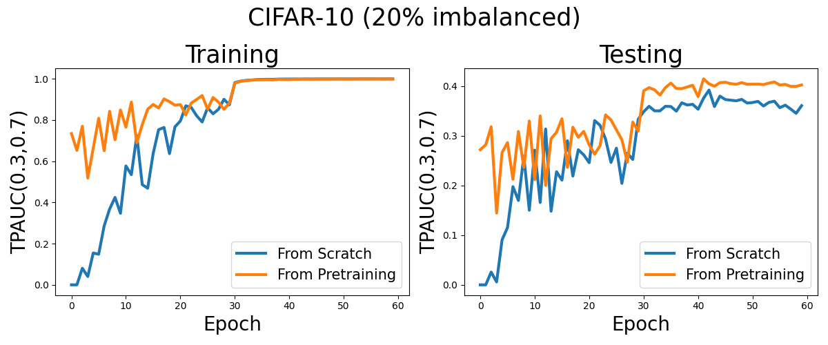
Visualization
Now, let’s see the learning curves for optimizing two way pAUC from scratch and from a pretrained model with cross entropy loss.
import matplotlib.pyplot as plt
import numpy as np

tr_tpAUC=[0.7340686421865071, 0.6523861417725976, 0.7697571757554482, 0.5181640862209829, 0.6632382487913021, 0.8082231370883574, 0.6509505406652053, 0.8419906017793952, 0.7042755724457082, 0.8485929759094291, 0.7652266175576936, 0.8868674039937814, 0.6897615571140835, 0.7768915847106662, 0.8523286213213361, 0.8752236481519994, 0.8581668457369729, 0.9021540891388055, 0.8892498033262324, 0.8716549717783728, 0.8747909107228096, 0.8243974955960515, 0.8819449923909647, 0.89989779260777, 0.9189142622615254, 0.8526040037279257, 0.9091358833770271, 0.8867607782454089, 0.8518731606635959, 0.8822833594960255, 0.9782023583634041, 0.9876358422173004, 0.9909971902527791, 0.9930102103870361, 0.9949333159065591, 0.9949216118874699, 0.9953726790912358, 0.9942961672503617, 0.997483689257653, 0.9965499735645696, 0.9962329244942777, 0.9977584491100356, 0.9976834402217404, 0.9982931164501517, 0.9977569194054131, 0.9983236393935511, 0.9982740129296326, 0.9983406262297669, 0.99876796522462, 0.9988299360490974, 0.9984605657445348, 0.9982824796668458, 0.9989244575649622, 0.9989117396718792, 0.998685361175001, 0.9987890609186011, 0.9991992885663972, 0.9987879047465028, 0.9987802206488635, 0.998913055929345]
te_tpAUC=[0.2720835555555555, 0.28182399999999996, 0.318144, 0.14448533333333333, 0.26637955555555554, 0.2863466666666667, 0.21235022222222222, 0.3087377777777778, 0.2363608888888889, 0.3297991111111111, 0.21162666666666666, 0.3400444444444444, 0.20017066666666666, 0.29414577777777773, 0.30727644444444446, 0.3343911111111111, 0.2363608888888889, 0.3173546666666667, 0.29697244444444443, 0.30892444444444445, 0.281632, 0.26309688888888894, 0.27994311111111114, 0.34215288888888895, 0.33189688888888885, 0.3119537777777778, 0.29198222222222225, 0.24688355555555558, 0.3276017777777777, 0.3095964444444444, 0.39057600000000003, 0.3969288888888889, 0.39256888888888886, 0.3820568888888889, 0.39707555555555557, 0.4060711111111111, 0.39528977777777774, 0.39492800000000006, 0.3983306666666666, 0.401728, 0.37883022222222223, 0.4146986666666667, 0.40477155555555555, 0.3997706666666666, 0.40691555555555553, 0.4078577777777778, 0.40501511111111116, 0.4037084444444444, 0.40711288888888886, 0.403744, 0.40399288888888885, 0.4041048888888889, 0.4031502222222223, 0.4060248888888889, 0.40843022222222225, 0.40232711111111114, 0.40354222222222225, 0.39950755555555556, 0.39955555555555555, 0.4024408888888889]
tr_tpAUC_scratch = [0.0, 0.0, 0.08050213763769921, 0.040334006379650914, 0.15452126257408305, 0.14852208121507784, 0.285387270694609, 0.3671972524228209, 0.42439337962338103, 0.3470672912083037, 0.57707256655478, 0.5347993927570692, 0.7244398719715495, 0.4864689355055898, 0.4687417578269827, 0.636698478356565, 0.7529223050215363, 0.7638683198955304, 0.6367875213954094, 0.7665590614330088, 0.7952058665808703, 0.8687836539463781, 0.8606273044733329, 0.8203095645457442, 0.7905463418323486, 0.8590389997126289, 0.8301345282721786, 0.8518168284015063, 0.9005089985408041, 0.8737030239272128, 0.9813676285046156, 0.9884804881906448, 0.992134579001453, 0.9937827023278047, 0.9961085381637468, 0.9967696284760136, 0.9973916935331416, 0.9972957668234957, 0.9982831022210528, 0.9987787443060302, 0.9986975810247185, 0.9989840982579795, 0.9986465849415449, 0.9992968161297178, 0.9988526325967533, 0.9991434098795156, 0.999431963754396, 0.9993364639390634, 0.9992874155611944, 0.9993348630853888, 0.9995505959053294, 0.9996459801034523, 0.9993523301777069, 0.9997270188739226, 0.9995369886490936, 0.9996679651605858, 0.9995451441092036, 0.9993488616614113, 0.9996902348139285, 0.9995364461375705]
te_tpAUC_scratch = [0.0, 0.0, 0.025589333333333335, 0.005740444444444445, 0.09052355555555555, 0.11532088888888889, 0.19768000000000002, 0.16982044444444444, 0.25902933333333333, 0.15017066666666665, 0.27112888888888886, 0.16573333333333334, 0.31376533333333334, 0.14812622222222221, 0.22768533333333335, 0.2108071111111111, 0.29003555555555555, 0.21898133333333336, 0.27193955555555555, 0.2615911111111111, 0.2459022222222222, 0.3306702222222222, 0.3210435555555555, 0.29353955555555555, 0.2464088888888889, 0.27508622222222223, 0.20425244444444446, 0.2650702222222222, 0.2524053333333333, 0.3334506666666667, 0.34853155555555554, 0.35939733333333335, 0.35027911111111104, 0.35027555555555556, 0.3594773333333333, 0.3589315555555555, 0.3496568888888889, 0.3664924444444444, 0.3620444444444445, 0.36339733333333335, 0.3535128888888889, 0.3757048888888889, 0.39203733333333335, 0.35895466666666664, 0.3799253333333333, 0.3730328888888889, 0.37171199999999993, 0.37044799999999994, 0.3733608888888889, 0.3659644444444444, 0.36706666666666665, 0.36921244444444445, 0.3599911111111111, 0.36727466666666664, 0.36972977777777777, 0.35660977777777775, 0.36172977777777776, 0.353872, 0.345256, 0.3606755555555555]

fig, (ax0, ax1) = plt.subplots(1, 2, figsize=(12,5))
plt.suptitle('CIFAR-10 (20% imbalanced)',fontsize=25)

x=np.arange(len(tr_tpAUC))
ax0.plot(x, tr_tpAUC_scratch,  label='From Scratch', linewidth=3)
ax0.plot(x, tr_tpAUC,  label='From Pretraining', linewidth=3)
ax0.set_title('Training',fontsize=25)
ax1.plot(x, te_tpAUC_scratch, label='From Scratch', linewidth=3)
ax1.plot(x, te_tpAUC, label='From Pretraining', linewidth=3)
ax1.set_title('Testing',fontsize=25)

ax0.legend(fontsize=15)
ax1.legend(fontsize=15)
ax0.set_ylabel('TPAUC(0.3,0.7)', fontsize=20)
ax0.set_xlabel('Epoch', fontsize=20)
ax1.set_ylabel('TPAUC(0.3,0.7)', fontsize=20)
ax1.set_xlabel('Epoch', fontsize=20)

plt.tight_layout()