Optimizing Two-Way partial AUC on Imbalanced CIFAR10 Dataset (STACO)
Introduction
In this tutorial, we will learn how to quickly train a ResNet18 model by optimizing two-way partial AUC (TPAUC) score using our novel tpAUC_CVaR_Loss and STACO optimizer [Ref] method on a binary image classification task on Cifar10. After completion of this tutorial, you should be able to use LibAUC to train your own models on your own datasets.
Reference:
If you find this tutorial helpful in your work, please cite our library paper and the following papers:
@article{
zhou2025stochastic,
title={Stochastic Primal-Dual Double Block-Coordinate for Two-way Partial {AUC} Maximization},
author={Linli Zhou and Bokun Wang and My T. Thai and Tianbao Yang},
journal={Transactions on Machine Learning Research},
issn={2835-8856},
year={2025},
url={https://openreview.net/forum?id=M3kibBFP4q},
note={}
}
Install LibAUC
Let’s start with installing our library here. In this tutorial, we will use the lastest version for LibAUC by using pip install -U.
!pip install -U libauc
Importing LibAUC
Import required libraries to use
from libauc.models import resnet18
from libauc.datasets import CIFAR10
from libauc.losses import tpAUC_CVaR_loss
from libauc.optimizers import STACO
from libauc.utils import ImbalancedDataGenerator
from libauc.sampler import DualSampler # data resampling (for binary class)
from libauc.metrics import pauc_roc_score

import torch
from PIL import Image
import numpy as np
import torchvision.transforms as transforms
from torch.utils.data import Dataset
import torch.nn as nn
Reproducibility
The following function set_all_seeds limits the number of sources
of randomness behaviors, such as model initialization, data shuffling,
etcs. However, completely reproducible results are not guaranteed
across PyTorch releases
[Ref].
def set_all_seeds(SEED):
   # REPRODUCIBILITY
   np.random.seed(SEED)
   torch.manual_seed(SEED)
   torch.cuda.manual_seed(SEED)
   torch.backends.cudnn.deterministic = True
   torch.backends.cudnn.benchmark = False
set_all_seeds(2023)
Image Dataset
Now we define the data input pipeline such as data augmentations. In this tutorials, we use RandomCrop, RandomHorizontalFlip. The pos_index_map helps map global index to local index for reducing memory cost in loss function since we only need to track the indices for positive samples.
class ImageDataset(Dataset):
  def __init__(self, images, targets, image_size=32, crop_size=30, mode='train'):
    self.images = images.astype(np.uint8)
    self.targets = targets
    self.mode = mode
    self.transform_train = transforms.Compose([
                            transforms.ToTensor(),
                            transforms.RandomCrop((crop_size, crop_size), padding=None),
                            transforms.RandomHorizontalFlip(),
                            transforms.Resize((image_size, image_size)),
                            ])
    self.transform_test = transforms.Compose([
                          transforms.ToTensor(),
                          transforms.Resize((image_size, image_size)),
                            ])

    # for loss function
    self.pos_indices = np.flatnonzero(targets==1)
    self.pos_index_map = {}
    for i, idx in enumerate(self.pos_indices):
        self.pos_index_map[idx] = i

  def __len__(self):
      return len(self.images)

  def __getitem__(self, idx):
      image = self.images[idx]
      target = self.targets[idx]
      image = Image.fromarray(image.astype('uint8'))
      if self.mode == 'train':
          idx = self.pos_index_map[idx] if idx in self.pos_indices else -1
          image = self.transform_train(image)
      else:
          image = self.transform_test(image)
      return image, target, idx
HyperParameters
# HyperParameters
SEED = 123
batch_size = 64
total_epochs = 60
weight_decay = 1e-4
lr = 1e-3
decay_epochs = [20, 40]
decay_factor = 10

# TPR is higher than 1-theta_0, FPR is lower than theta_1
theta_0 = theta_1 = 0.5
# alpha: the step size for dual variable y, beta_0: the step size for s, beta_1: the step size for s'
alpha = beta_0 = beta_1 = 1e-3

sampling_rate = 0.5
num_pos = round(sampling_rate*batch_size)
num_neg = batch_size - num_pos
Loading datasets
train_data, train_targets = CIFAR10(root='./data', train=True).as_array()
test_data, test_targets  = CIFAR10(root='./data', train=False).as_array()

imratio = 0.2
g = ImbalancedDataGenerator(shuffle=True, verbose=True, random_seed=0)
(train_images, train_labels) = g.transform(train_data, train_targets, imratio=imratio)
(test_images, test_labels) = g.transform(test_data, test_targets, imratio=0.5)

trainSet = ImageDataset(train_images, train_labels)
testSet = ImageDataset(test_images, test_labels, mode = 'test')
sampler = DualSampler(dataset=trainSet, batch_size=batch_size, labels=train_labels, shuffle=True, sampling_rate=sampling_rate)
trainloader =  torch.utils.data.DataLoader(trainSet, sampler=sampler, batch_size=batch_size, shuffle=False, num_workers=0)
testloader =  torch.utils.data.DataLoader(testSet, batch_size=32, num_workers=0, shuffle=False)
Files already downloaded and verified
Files already downloaded and verified
#SAMPLES: 31250, CLASS 0.0 COUNT: 25000, CLASS RATIO: 0.8000
#SAMPLES: 31250, CLASS 1.0 COUNT: 6250, CLASS RATIO: 0.2000
#SAMPLES: 10000, CLASS 1.0 COUNT: 5000, CLASS RATIO: 0.5000
#SAMPLES: 10000, CLASS 0.0 COUNT: 5000, CLASS RATIO: 0.5000
Creating models & TPAUC Optimizer
set_all_seeds(SEED)
model = resnet18(pretrained=False, num_classes=1, last_activation=None)

model = model.cuda()

# Initialize the loss function and optimizer
loss_fn = tpAUC_CVaR_loss(data_length=sampler.pos_len, alpha=alpha, beta_0=beta_0, beta_1=beta_1, theta_0=theta_0, theta_1=theta_1)
optimizer = STACO(model.parameters(), loss_fn=loss_fn, mode='adam', lr=lr, weight_decay=weight_decay)
Training
Now it’s time for training.
print ('Start Training')
print ('-'*30)

tr_tpAUC=[]
te_tpAUC=[]

for epoch in range(total_epochs):
    if epoch in decay_epochs:
        optimizer.update_lr(decay_factor=decay_factor)
        loss_fn.alpha /= decay_factor
        loss_fn.beta_0 /= decay_factor
        loss_fn.beta_1 /= decay_factor

    train_loss = 0
    model.train()
    for idx, data in enumerate(trainloader):
        train_data, train_labels, index = data
        train_data, train_labels = train_data.cuda(), train_labels.cuda()
        y_pred = model(train_data)
        loss = loss_fn(y_pred, train_labels, index[:num_pos])
        train_loss = train_loss  + loss.cpu().detach().numpy()
        optimizer.zero_grad()
        loss.backward()
        optimizer.step()
    train_loss = train_loss/(idx+1)

    # evaluation
    model.eval()
    with torch.no_grad():
        train_pred = []
        train_true = []
        for jdx, data in enumerate(trainloader):
            train_data, train_labels,_ = data
            train_data = train_data.cuda()
            y_pred = model(train_data)
            y_prob = torch.sigmoid(y_pred)
            train_pred.append(y_prob.cpu().detach().numpy())
            train_true.append(train_labels.numpy())
        train_true = np.concatenate(train_true)
        train_pred = np.concatenate(train_pred)
        single_train_auc =  pauc_roc_score(train_true, train_pred, max_fpr = 0.3, min_tpr=0.7)

        test_pred = []
        test_true = []
        for jdx, data in enumerate(testloader):
            test_data, test_labels, _ = data
            test_data = test_data.cuda()
            y_pred = model(test_data)
            y_prob = torch.sigmoid(y_pred)
            test_pred.append(y_prob.cpu().detach().numpy())
            test_true.append(test_labels.numpy())
        test_true = np.concatenate(test_true)
        test_pred = np.concatenate(test_pred)
        single_test_auc =  pauc_roc_score(test_true, test_pred, max_fpr = 0.3, min_tpr=0.7)
        print('Epoch=%s, Loss=%0.4f, Train_tpAUC(0.3,0.7)=%.4f, Test_tpAUC(0.3,0.7)=%.4f, lr=%.4f'%(epoch, train_loss, single_train_auc, single_test_auc, optimizer.lr))

        tr_tpAUC.append(single_train_auc)
        te_tpAUC.append(single_test_auc)
Start Training
------------------------------
Epoch=0, Loss=0.7769, Train_tpAUC(0.3,0.7)=0.0083, Test_tpAUC(0.3,0.7)=0.0027, lr=0.0010
Epoch=1, Loss=0.5561, Train_tpAUC(0.3,0.7)=0.0003, Test_tpAUC(0.3,0.7)=0.0000, lr=0.0010
Epoch=2, Loss=0.4426, Train_tpAUC(0.3,0.7)=0.0901, Test_tpAUC(0.3,0.7)=0.0508, lr=0.0010
Epoch=3, Loss=0.3564, Train_tpAUC(0.3,0.7)=0.1696, Test_tpAUC(0.3,0.7)=0.1078, lr=0.0010
Epoch=4, Loss=0.2897, Train_tpAUC(0.3,0.7)=0.3645, Test_tpAUC(0.3,0.7)=0.1791, lr=0.0010
Epoch=5, Loss=0.2330, Train_tpAUC(0.3,0.7)=0.3899, Test_tpAUC(0.3,0.7)=0.1958, lr=0.0010
Epoch=6, Loss=0.1927, Train_tpAUC(0.3,0.7)=0.4758, Test_tpAUC(0.3,0.7)=0.2084, lr=0.0010
Epoch=7, Loss=0.1622, Train_tpAUC(0.3,0.7)=0.3806, Test_tpAUC(0.3,0.7)=0.1483, lr=0.0010
Epoch=8, Loss=0.1318, Train_tpAUC(0.3,0.7)=0.3751, Test_tpAUC(0.3,0.7)=0.0954, lr=0.0010
Epoch=9, Loss=0.1049, Train_tpAUC(0.3,0.7)=0.6161, Test_tpAUC(0.3,0.7)=0.1791, lr=0.0010
Epoch=10, Loss=0.0851, Train_tpAUC(0.3,0.7)=0.6697, Test_tpAUC(0.3,0.7)=0.2554, lr=0.0010
Epoch=11, Loss=0.0735, Train_tpAUC(0.3,0.7)=0.6783, Test_tpAUC(0.3,0.7)=0.2324, lr=0.0010
Epoch=12, Loss=0.0570, Train_tpAUC(0.3,0.7)=0.6791, Test_tpAUC(0.3,0.7)=0.2125, lr=0.0010
Epoch=13, Loss=0.0509, Train_tpAUC(0.3,0.7)=0.7166, Test_tpAUC(0.3,0.7)=0.1990, lr=0.0010
Epoch=14, Loss=0.0432, Train_tpAUC(0.3,0.7)=0.6712, Test_tpAUC(0.3,0.7)=0.2173, lr=0.0010
Epoch=15, Loss=0.0366, Train_tpAUC(0.3,0.7)=0.6469, Test_tpAUC(0.3,0.7)=0.2462, lr=0.0010
Epoch=16, Loss=0.0299, Train_tpAUC(0.3,0.7)=0.8008, Test_tpAUC(0.3,0.7)=0.3238, lr=0.0010
Epoch=17, Loss=0.0250, Train_tpAUC(0.3,0.7)=0.7510, Test_tpAUC(0.3,0.7)=0.2185, lr=0.0010
Epoch=18, Loss=0.0211, Train_tpAUC(0.3,0.7)=0.7333, Test_tpAUC(0.3,0.7)=0.2713, lr=0.0010
Epoch=19, Loss=0.0182, Train_tpAUC(0.3,0.7)=0.7187, Test_tpAUC(0.3,0.7)=0.2233, lr=0.0010
Reducing learning rate to 0.00010 @ T=15620!
Epoch=20, Loss=0.0079, Train_tpAUC(0.3,0.7)=0.9566, Test_tpAUC(0.3,0.7)=0.3584, lr=0.0001
Epoch=21, Loss=0.0041, Train_tpAUC(0.3,0.7)=0.9705, Test_tpAUC(0.3,0.7)=0.3665, lr=0.0001
Epoch=22, Loss=0.0028, Train_tpAUC(0.3,0.7)=0.9784, Test_tpAUC(0.3,0.7)=0.3786, lr=0.0001
Epoch=23, Loss=0.0022, Train_tpAUC(0.3,0.7)=0.9817, Test_tpAUC(0.3,0.7)=0.3660, lr=0.0001
Epoch=24, Loss=0.0019, Train_tpAUC(0.3,0.7)=0.9878, Test_tpAUC(0.3,0.7)=0.3658, lr=0.0001
Epoch=25, Loss=0.0016, Train_tpAUC(0.3,0.7)=0.9879, Test_tpAUC(0.3,0.7)=0.3671, lr=0.0001
Epoch=26, Loss=0.0014, Train_tpAUC(0.3,0.7)=0.9880, Test_tpAUC(0.3,0.7)=0.3684, lr=0.0001
Epoch=27, Loss=0.0012, Train_tpAUC(0.3,0.7)=0.9902, Test_tpAUC(0.3,0.7)=0.3505, lr=0.0001
Epoch=28, Loss=0.0013, Train_tpAUC(0.3,0.7)=0.9921, Test_tpAUC(0.3,0.7)=0.3423, lr=0.0001
Epoch=29, Loss=0.0011, Train_tpAUC(0.3,0.7)=0.9916, Test_tpAUC(0.3,0.7)=0.3578, lr=0.0001
Epoch=30, Loss=0.0011, Train_tpAUC(0.3,0.7)=0.9904, Test_tpAUC(0.3,0.7)=0.3379, lr=0.0001
Epoch=31, Loss=0.0011, Train_tpAUC(0.3,0.7)=0.9933, Test_tpAUC(0.3,0.7)=0.3677, lr=0.0001
Epoch=32, Loss=0.0009, Train_tpAUC(0.3,0.7)=0.9916, Test_tpAUC(0.3,0.7)=0.3506, lr=0.0001
Epoch=33, Loss=0.0011, Train_tpAUC(0.3,0.7)=0.9921, Test_tpAUC(0.3,0.7)=0.3405, lr=0.0001
Epoch=34, Loss=0.0010, Train_tpAUC(0.3,0.7)=0.9917, Test_tpAUC(0.3,0.7)=0.3405, lr=0.0001
Epoch=35, Loss=0.0009, Train_tpAUC(0.3,0.7)=0.9919, Test_tpAUC(0.3,0.7)=0.3500, lr=0.0001
Epoch=36, Loss=0.0010, Train_tpAUC(0.3,0.7)=0.9917, Test_tpAUC(0.3,0.7)=0.3385, lr=0.0001
Epoch=37, Loss=0.0009, Train_tpAUC(0.3,0.7)=0.9922, Test_tpAUC(0.3,0.7)=0.3134, lr=0.0001
Epoch=38, Loss=0.0010, Train_tpAUC(0.3,0.7)=0.9916, Test_tpAUC(0.3,0.7)=0.3365, lr=0.0001
Epoch=39, Loss=0.0009, Train_tpAUC(0.3,0.7)=0.9928, Test_tpAUC(0.3,0.7)=0.3325, lr=0.0001
Reducing learning rate to 0.00001 @ T=31240!
Epoch=40, Loss=0.0006, Train_tpAUC(0.3,0.7)=0.9965, Test_tpAUC(0.3,0.7)=0.3450, lr=0.0000
Epoch=41, Loss=0.0004, Train_tpAUC(0.3,0.7)=0.9973, Test_tpAUC(0.3,0.7)=0.3559, lr=0.0000
Epoch=42, Loss=0.0003, Train_tpAUC(0.3,0.7)=0.9985, Test_tpAUC(0.3,0.7)=0.3526, lr=0.0000
Epoch=43, Loss=0.0003, Train_tpAUC(0.3,0.7)=0.9986, Test_tpAUC(0.3,0.7)=0.3488, lr=0.0000
Epoch=44, Loss=0.0002, Train_tpAUC(0.3,0.7)=0.9987, Test_tpAUC(0.3,0.7)=0.3589, lr=0.0000
Epoch=45, Loss=0.0002, Train_tpAUC(0.3,0.7)=0.9990, Test_tpAUC(0.3,0.7)=0.3578, lr=0.0000
Epoch=46, Loss=0.0002, Train_tpAUC(0.3,0.7)=0.9990, Test_tpAUC(0.3,0.7)=0.3590, lr=0.0000
Epoch=47, Loss=0.0002, Train_tpAUC(0.3,0.7)=0.9993, Test_tpAUC(0.3,0.7)=0.3574, lr=0.0000
Epoch=48, Loss=0.0002, Train_tpAUC(0.3,0.7)=0.9991, Test_tpAUC(0.3,0.7)=0.3645, lr=0.0000
Epoch=49, Loss=0.0001, Train_tpAUC(0.3,0.7)=0.9991, Test_tpAUC(0.3,0.7)=0.3697, lr=0.0000
Epoch=50, Loss=0.0002, Train_tpAUC(0.3,0.7)=0.9991, Test_tpAUC(0.3,0.7)=0.3672, lr=0.0000
Epoch=51, Loss=0.0001, Train_tpAUC(0.3,0.7)=0.9994, Test_tpAUC(0.3,0.7)=0.3669, lr=0.0000
Epoch=52, Loss=0.0001, Train_tpAUC(0.3,0.7)=0.9994, Test_tpAUC(0.3,0.7)=0.3709, lr=0.0000
Epoch=53, Loss=0.0001, Train_tpAUC(0.3,0.7)=0.9996, Test_tpAUC(0.3,0.7)=0.3621, lr=0.0000
Epoch=54, Loss=0.0001, Train_tpAUC(0.3,0.7)=0.9997, Test_tpAUC(0.3,0.7)=0.3673, lr=0.0000
Epoch=55, Loss=0.0001, Train_tpAUC(0.3,0.7)=0.9994, Test_tpAUC(0.3,0.7)=0.3683, lr=0.0000
Epoch=56, Loss=0.0001, Train_tpAUC(0.3,0.7)=0.9997, Test_tpAUC(0.3,0.7)=0.3755, lr=0.0000
Epoch=57, Loss=0.0001, Train_tpAUC(0.3,0.7)=0.9998, Test_tpAUC(0.3,0.7)=0.3776, lr=0.0000
Epoch=58, Loss=0.0001, Train_tpAUC(0.3,0.7)=0.9996, Test_tpAUC(0.3,0.7)=0.3722, lr=0.0000
Epoch=59, Loss=0.0001, Train_tpAUC(0.3,0.7)=0.9999, Test_tpAUC(0.3,0.7)=0.3707, lr=0.0000
Visualization
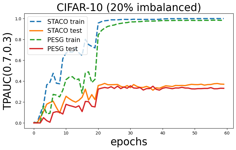
Now, let’s see the change of two-way partial AUC scores on training and testing set and compare it with AUCM method.
import matplotlib.pyplot as plt
plt.rcParams["figure.figsize"] = (9,5)
x=np.arange(60)
aucm_tr_tpAUC = [0.0, 0.0036274632780175535, 0.005047971892709222, 0.16224877002854712, 0.08772204107278256, 0.09231572626711304, 0.2732654643710093, 0.26647582593555136, 0.24948327111467297, 0.3138958243403896, 0.41470878408333095, 0.43854233806173326, 0.44279415206018125, 0.41232459713094294, 0.42158369465786594, 0.28455608967939594, 0.47755676075725645, 0.4896781046120168, 0.3863189337375359, 0.41758365936793596, 0.842293465507402, 0.8849664436167597, 0.908744785930645, 0.925100663457797, 0.9326945885667315, 0.9383691079068582, 0.9493701298918441, 0.953469756067609, 0.959401363614275, 0.9611639035102166, 0.9687268876750703, 0.96784177567828, 0.9702642497143897, 0.9702752956047458, 0.9733664551144465, 0.9760006331554156, 0.9760579703978677, 0.9755799377033129, 0.9770459817114208, 0.9787550086264667, 0.9813317160205113, 0.9802740408912104, 0.9814502948096553, 0.9811205278462805, 0.9821393644867049, 0.9823378881296415, 0.9827693626631546, 0.9815768245053843, 0.9835002857701681, 0.9825182242961066, 0.9819347131316462, 0.9819089304938505, 0.9819178330190087, 0.9830069649230193, 0.982775401438961, 0.9835906895346361, 0.9843369096878757, 0.9844427527966737, 0.9829346774859711, 0.9838700118199921]
aucm_te_tpAUC = [0.0, 0.000301777777777778, 0.0, 0.050526666666666664, 0.022042666666666665, 0.006600444444444444, 0.09903022222222221, 0.10774866666666666, 0.1029888888888889, 0.08559822222222221, 0.17839955555555553, 0.16736266666666666, 0.1591968888888889, 0.14970355555555553, 0.16401288888888887, 0.10874133333333333, 0.2060488888888889, 0.20340622222222224, 0.15917866666666666, 0.15321466666666667, 0.3240817777777778, 0.3328191111111111, 0.33990511111111105, 0.33390533333333333, 0.3470675555555556, 0.3300217777777778, 0.35229422222222223, 0.32868844444444445, 0.34444044444444444, 0.33212177777777785, 0.3557311111111111, 0.33471155555555554, 0.332584, 0.3388742222222223, 0.31508044444444444, 0.3285328888888889, 0.32913555555555557, 0.35162800000000005, 0.32234244444444443, 0.31436844444444445, 0.331578888888889, 0.3387742222222222, 0.3338368888888889, 0.3277377777777778, 0.335048, 0.3345755555555555, 0.34122044444444444, 0.3344044444444444, 0.33397066666666664, 0.32639111111111113, 0.3255946666666667, 0.3287395555555556, 0.3287168888888889, 0.33072799999999997, 0.3306648888888889, 0.33826266666666666, 0.3271982222222222, 0.3275493333333333, 0.33227422222222225, 0.33158488888888893]
plt.figure()
plt.plot(x, tr_tpAUC, linestyle='--', label='STACO train', linewidth=3)
plt.plot(x, te_tpAUC, label='STACO test', linewidth=3)
plt.plot(x, aucm_tr_tpAUC, linestyle='--', label='PESG train', linewidth=3)
plt.plot(x, aucm_te_tpAUC, label='PESG test', linewidth=3)
plt.title('CIFAR-10 (20% imbalanced)',fontsize=25)
plt.legend(fontsize=15)
plt.ylabel('TPAUC(0.7,0.3)',fontsize=25)
plt.xlabel('epochs',fontsize=25)